← All examples

Example · Python · Version 2.0.0

Kernel Flow BCI Real-Time Visualization

Reconstruct Kernel Flow fNIRS moments into 3D hemoglobin volumes with CuPy and render them interactively with VTK on Holoscan 5.x.

Run locally ▶

Authors	Holoscan Team (NVIDIA), Kernel Team (Kernel), Mimi Liao (NVIDIA), Tom Birdsong (NVIDIA), Julien Dubois (Kernel), Victor Szczepanski (Kernel), Gabe Lerner (Kernel)
Supported platforms	x86_64, aarch64
Language	Python
Version	2.0.0
Compatibility	HSDK 5.0
Contribution level	Level 2 · Quality code
Source	holoscan-applications ↗

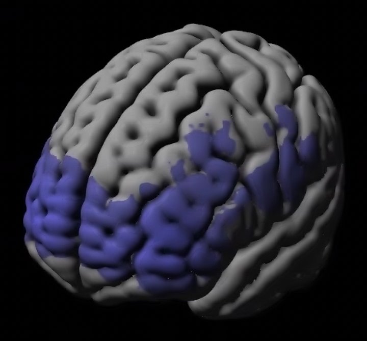
This application reconstructs brain activity from Kernel Flow functional near-infrared spectroscopy (fNIRS) data and shows it on an interactive 3D brain. It replays a recorded SNIRF file or streams from a Kernel Flow headset, solves the inverse problem on the GPU with CuPy, and renders the oxygenated-hemoglobin changes on an anatomical brain model with VTK. Every operator is a Holoscan SDK 5.x Python operator.

Overview

This application demonstrates real-time source reconstruction and 3D visualization for brain-computer interface (BCI) pipelines built with NVIDIA Holoscan. The Holoscan 4.x version was developed with Kernel and tested on an NVIDIA Jetson Thor paired with a Kernel Flow 2 headset. A recorded dataset and a replayer let you build and experiment with visualization and classification pipelines without access to the hardware.

The application processes streaming moments from the distribution of time-of-flight histograms, read from a shared near-infrared spectroscopy format (SNIRF) recording. It combines the moments with the sensors' spatial geometry and an average anatomical head model to produce source-reconstructed outputs similar to previously published work.

Background

Kernel Flow is a multimodal non-invasive brain measurement system. It combines the relatively high resolution of time-domain functional near-infrared spectroscopy (TD-fNIRS) with the fast temporal resolution of electroencephalography (EEG) in a compact and scalable form factor that enables a new class of non-invasive BCI applications.

The differentiating technology behind Kernel Flow is its time-resolved detectors and high-speed laser drivers. Short (~100 ps) pulses of near-infrared laser light (690 nm and 905 nm) are emitted into the user's head with a repetition rate of 20 MHz. The photons in these pulses scatter through the scalp, skull, and cerebrospinal fluid before reaching the brain and then scattering back out. When the photons emerge from the scalp, single-photon-sensitive detectors timestamp exactly how long each photon took to traverse the head. That time is proportional to the path length the photon traveled and the average depth it reached.

This simulation shows the relationship between photon scattering paths (black lines) and the measured time of flight (blue sections):

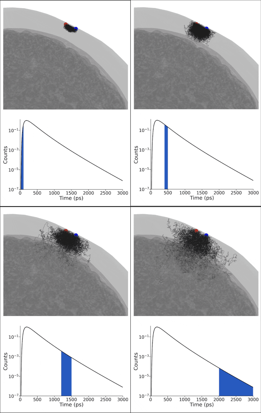
Later times correspond to photons that traveled farther into the tissue. Kernel Flow timestamps over 10 billion individual photons each second; after compression, it produces about 1 GB of data per minute.

As the photons scatter through the tissue, many are absorbed by cells and molecules. The wavelengths used are particularly sensitive to hemoglobin in its two states, oxyhemoglobin and deoxyhemoglobin. This makes it possible to follow the locations in the brain that are demanding and consuming oxygen, an indirect measure of neuronal activity. The same biophysical principles are behind the pulse oximeters in smart watches and finger-clip sensors. For more detail on the biophysics, see this review article.

The Kernel Flow headset combines 120 laser sources and 240 custom sensors to collect over 3000 measurement paths that criss-cross the head, at a frame rate of 4.75 Hz:

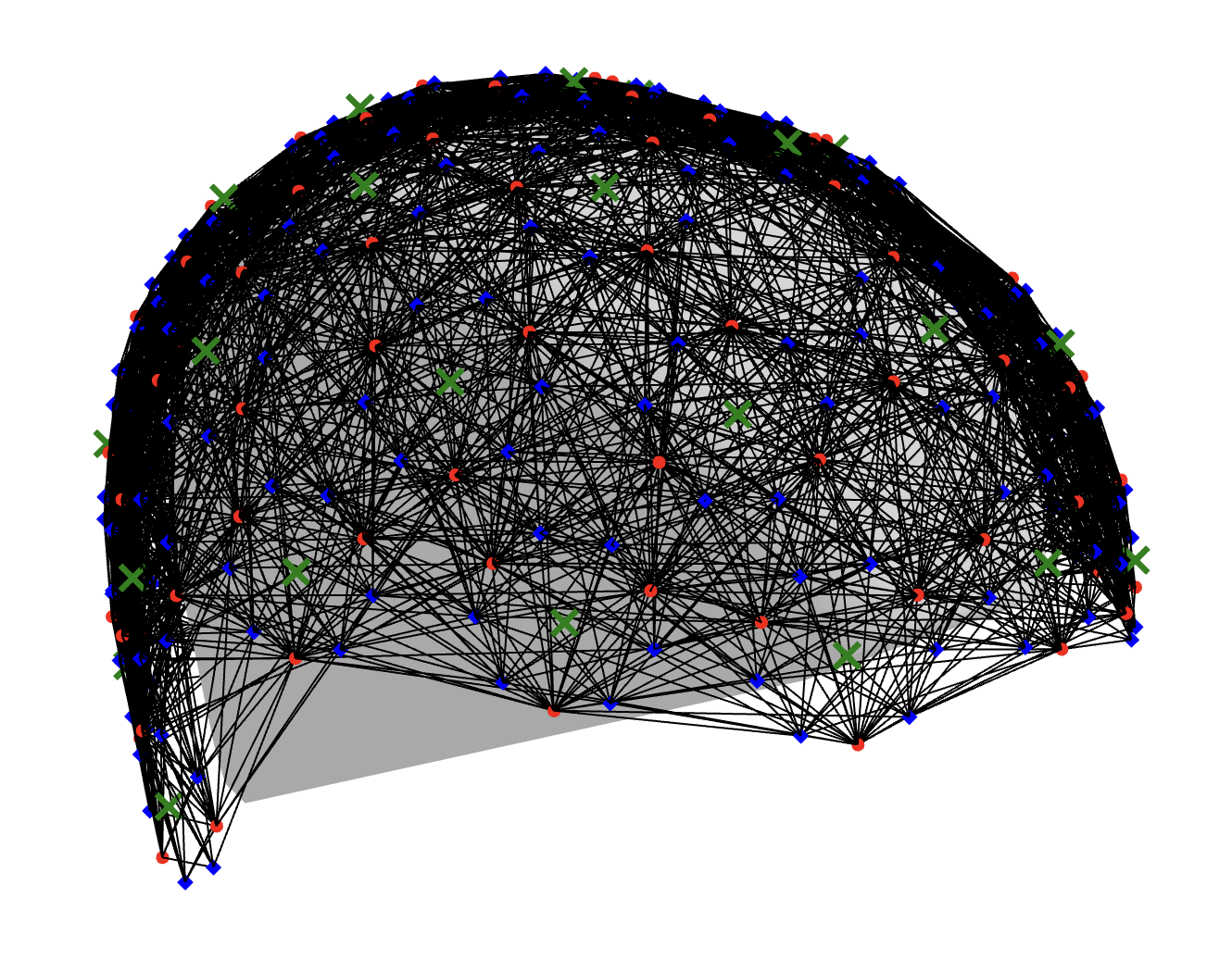
Each measurement path is a "channel", and the measurement is made in sensor space, from the perspective of the detector. For a more anatomical representation, the sensor-space data is commonly transformed into source space, where the changes in hemoglobin concentration likely occurred in the brain, by solving an inverse problem known as source reconstruction. This inverse problem requires computationally expensive but highly parallelizable modeling. This application solves it on the GPU in real time, at the native 4.75 Hz frame rate of Kernel Flow, and renders the result as a 3D volume.

Dependencies

• Linux on x86_64 or aarch64 with an NVIDIA GPU and a driver supporting CUDA 13.
• Python 3.12 and the packages in requirements.txt, including the Holoscan SDK 5.x Python Core (holoscan-core-cu13), CuPy, and VTK.
• An X display for the interactive window. Headless runs render offscreen with EGL.
• A Kernel Flow data source: a recorded SNIRF file (see Prepare the data) or a headset with Kortex (see Stream from a Kernel Flow headset).

The application Dockerfile installs these on a CUDA runtime image; the Holoscan CLI uses it for container builds and runs.

Prepare the data

holoscan build and holoscan run download the data into data/bci_visualization the first time (except in the ci mode). Pass --configure-args="-DHOLOHUB_DOWNLOAD_DATASETS=OFF" to skip the download. To prepare it by hand instead, from the repository root:

Bash

python3 applications/bci_visualization/prepare_data.py --output data/bci_visualization

This downloads a pinned revision of the Kernel sample dataset under the Apache License 2.0: the SNIRF recording (about 500 MB), the anatomy mask, and the reconstruction assets for the flow_2 headset, whose channel map covers every channel in this recording. Its Jacobian is 14.25 GB and is loaded into GPU memory, so the GPU needs more than 14.25 GB free.

The prepared dataset occupies about 14.8 GB on disk. Allow roughly 17–20 minutes for the initial download, based on an observed transfer; actual time depends on network throughput. Replacing an existing dataset with --force can temporarily require about 29 GB because each new file is downloaded before replacing the old copy.

Downloads use a 60-second network operation timeout and a two-hour deadline per file, including opening the connection and streaming the response. For slower networks, prepare manually with larger limits (in seconds):

Bash

python3 applications/bci_visualization/prepare_data.py --output data/bci_visualization \
  --network-timeout 120 --download-deadline 14400

The dataset contains:

• data.snirf: the recorded brain activity measurements.
• anatomy_labels_high_res.nii.gz: the brain tissue segmentation (skin, skull, CSF, gray matter, white matter).
• Reconstruction assets for one headset: the precomputed Jacobian, the channel map, and the voxel information.

The prepared folder has this structure:

Plain text

data/bci_visualization/
├── anatomy_labels_high_res.nii.gz      # Brain segmentation
├── data.snirf                          # SNIRF brain activity recording
├── extinction_coefficients_mua.csv     # Absorption coefficients for HbO/HbR
├── flow_channel_map.json               # Source-detector channel mapping
├── flow_mega_jacobian.npy              # Precomputed sensitivity matrix (channels → voxels)
└── voxel_info/                         # Voxel geometry and optical properties
    ├── affine.npy                      # 4x4 affine transformation matrix
    ├── idxs_significant_voxels.npy     # Indices of voxels with sufficient sensitivity
    ├── ijk.npy                         # Voxel coordinates in volume space
    ├── mua.npy                         # Absorption coefficient per voxel
    ├── musp.npy                        # Reduced scattering coefficient per voxel
    ├── resolution.npy                  # Voxel resolution (mm)
    ├── wavelengths.npy                 # Measurement wavelengths (690 nm, 905 nm)
    └── xyz.npy                         # Voxel coordinates in anatomical space (mm)

Pick another headset's assets with --headset when replaying a matching recording. Each file is checked against the SHA-256 checksums in dataset_checksums.json: files that match are kept, and missing or mismatched files are downloaded again. Pass --force to download every file. More recordings are available on OpenNeuro.

Run

Bash

holoscan run bci_visualization

Drag with the left mouse button to rotate, the right button or the wheel to zoom, and the middle button to pan. Close the window, or press q, to stop. The application also exits when the recording ends.

The headless mode renders offscreen and writes the last frame to bci_visualization.png. The ci mode replays a small generated dataset at the recording pace, so it needs a GPU but no data or display:

Bash

holoscan run bci_visualization headless
holoscan run bci_visualization ci

To run directly with Python, pass the data directory:

Bash

python3 applications/bci_visualization/python/bci_visualization.py --data data/bci_visualization

By default the replay runs as fast as the pipeline reconstructs frames. Add --replay-rate realtime to follow the recording's timestamps (4.75 Hz for Kernel Flow). --frames N stops after N samples; 0 replays all samples. Reconstruction requires at least two samples: the first captures the baseline and the next produces a volume. --frames 1 and recordings with fewer than two samples are rejected, including in compile-only mode. Run with --help for the other options.

Stream from a Kernel Flow headset

The live mode streams moments from a Flow headset through Kernel's Kortex service and the Kernel SDK (kernel-sdk, installed with the other requirements). Prepare the data for your headset with prepare_data.py --headset, start Kortex on the same machine, and run:

Bash

holoscan run bci_visualization live

The live mode mounts Kortex's /etc/kernel.com/kortex.json read-only into the container; if the file is missing, Docker refuses to start the container.

The application keeps the channels that are valid in the first sample, and stops with an error that lists unmapped channels if the headset's assets don't match. Samples are shown as they arrive; if reconstruction falls behind, the oldest waiting samples are dropped. The run continues until you close the window, or for --frames N samples. Device simulation also exits when its recording ends, with or without a window. The Kernel SDK reports errors to Kernel through Sentry unless SENTRY_DSN_SDK is empty, so the application sets it empty unless you set it yourself.

To try the live path without a headset, --source kernel --simulate-device streams the recording through the same code at its recorded rate, and --synthetic does the same on generated data:

Bash

python3 applications/bci_visualization/python/bci_visualization.py \
  --synthetic --source kernel --simulate-device

Pipeline

flowchart LR
    S[SNIRF replay or Kernel Flow] --> B[Build RHS]
    B --> N[Normalize]
    N --> R[Regularized solver]
    R --> C[Convert to voxels]
    C --> V[Voxel stream to volume]
    V --> W[VTK view]

The reconstruction steps transform sensor-space measurements into 3D brain activity maps:

1. Stream (StreamOperator) reads the SNIRF recording or the headset and emits the time-of-flight moments of each sample with its channel layout.
2. Build RHS builds the right-hand side of the inverse problem from the moments, using the channel map to select the matching Jacobian rows.
3. Normalize scales the moments and the Jacobian by fixed upper bounds.
4. Regularized solver solves the inverse problem on the GPU.
5. Convert to voxels maps the solution to voxel coordinates and converts it to oxygenated (HbO) and deoxygenated (HbR) hemoglobin changes.
6. Voxel stream to volume resamples the HbO changes onto the anatomy mask grid and scales them for display with a running minimum and maximum.

VTK view runs on its own 30 Hz clock and takes the newest volume, so the window stays responsive and interactive between reconstructed frames.

Visualization

By default the view colors a smoothed cortex surface with the activity averaged over the first 6 mm below it (--surface-depth-mm). Blue shows decreases, red shows increases, and gray shows baseline.

The surface view also darkens sulci, like the 4.x path-traced shading; --no-surface-texture turns that off.

--view volume ray casts the whole volume instead, as the 4.x application did. It uses VTK's GPU ray-cast mapper, limited to gray matter (label 3) and white matter (label 4) of the anatomy mask. The mask's other labels are skin (0), skull (1), CSF (2) and air (5). The transfer function follows the three layers of the 4.x application, over the displayed density range (−100 to 100 by default):

• Blue, opaque (lowest 40%): decreased oxygenated hemoglobin, from bright to dark blue.
• White, semi-transparent (40–60%): baseline tissue with no significant change.
• Red, opaque (highest 40%): increased oxygenated hemoglobin, from dark to bright red.

Tests

Bash

holoscan test bci_visualization

The data preparation test needs only Python. The other tests need the packages in requirements.txt; the solver and end-to-end tests also need a GPU. The interactive replay completion test additionally needs an X display (DISPLAY); it is skipped when no display is available. A virtual X server such as Xvfb can be used.

Changes from the Holoscan 4.x application

• The ClaraViz volume renderer and HoloViz window are replaced by a VTK operator that owns its window and mouse interaction. VTK reads host memory, so the surface view copies only the surface colors from the GPU for each displayed volume, while --view volume copies the whole volume for VTK's GPU ray-cast volume mapper.
• The rendering uses the 4.x colors and visible anatomy regions, without ClaraViz's path-traced lighting. functional near-infrared spectroscopy (fNIRS) data and shows it on an interactive 3D brain. It replays a recorded SNIRF file or streams from a Kernel Flow headset, solves the inverse problem on the GPU with CuPy, and renders the oxygenated-hemoglobin changes on

The render clock drains a depth-one queue of completed volumes. Input timestamps remain intact; slow reconstruction or initial scene setup does not expire the final frame.

Known limitation: multiple headsets and custom data

The standard sample workflow uses the Flow 2 dataset and flow_2 reconstruction assets. Dataset preparation writes to one shared directory and does not coordinate writes across build trees or detect manual changes to data after a successful build. Builds for different headsets that share HOLOHUB_DATA_DIR can overwrite each other's assets; concurrent preparation can mix files from different headsets. Use a separate HOLOHUB_DATA_DIR for each headset and do not prepare different headsets into the same directory concurrently. For manually supplied data, disable automatic downloads with --configure-args="-DHOLOHUB_DOWNLOAD_DATASETS=OFF" and provide a complete, matching set of recording and reconstruction assets via the application's --data option. Selecting another headset's assets does not replace the bundled Flow 2 recording with a matching recording.

Inherited limitations

The following limitations from the archived Holoscan 4.x application are deferred beyond this port:

• Display statistics require both extrema to be nonzero before initialization. Activity with only positive or only negative values alongside zero background remains hidden until a frame satisfies that condition. The archived code used the same condition, but could fail while updating uninitialized statistics; this port waits instead. See the archived normalizer.
• Voxel placement subtracts the minimum rounded IJK index without adjusting the affine translation. Custom grids with a nonzero minimum index can therefore shift activity relative to the anatomy. See the archived voxel conversion.
• The solver caches its regularized Hessian by wavelength index alone. Solving another dataset or changing --reg within the same Python process can reuse the wrong matrix and silently produce incorrect activity, even when the system dimensions match. Start a fresh process for each dataset or regularization setting; do not call the application repeatedly with different settings in one interpreter. See the archived solver cache.
• SNIRF replay defines its reference channel set from moment zero at wavelength zero. A measurement whose source/detector pair is absent from that set is assigned index -1 and overwrites the last reference channel, silently corrupting activity. Use recordings in which every measurement's source/detector pair is present in that reference set; verify this before replaying custom recordings. See the archived SNIRF channel mapping.
• A failed headset startup can leave the receiver thread and SDK connection active until process exit. The archived stream did not clean up after its first-sample timeout; this port also rejects a first sample with no valid channels without cleaning up the receiver. Exit the Python process after a startup failure, check the headset and Kortex service, then restart in a fresh process. Do not retry startup in the same interpreter. See the archived headset startup.

All examples →